茶桁.MAMT

2023-08-22发表AI 秘籍 / Python

先跟小伙伴们打个招呼，今天这节课呢，就是我们 Python 基础课程的最后一节课了。

在本节课之前，我们讲解了 Python 的基础，介绍了两个第三方库。而今天一样会介绍一个第三方库：Pandas。

虽然是最后一节课了，但是本节课的任务却是一点也不轻松。相比较而言，如果你以后从事的是数据治理和分析工作，那么本节课的内容可能会是你在今后工作中用到的最多的内容。我们需要学习行列索引的操作，数据的处理，数据的合并，多层索引，时间序列，数据的分组聚合（重点）。最后，我们会有一个案例的展示。

听着是不是很兴奋？那我们就开始吧。

在开始讲解 pandas 之前，我们讲解一些关于数据的小知识。

我们大部分人应该都用过 Excel 表格，而我们从数据库中拿到的数据，也基本上和 Excel 上的数据差不多，都是由行列组成的。可以直接导出为csv文件。

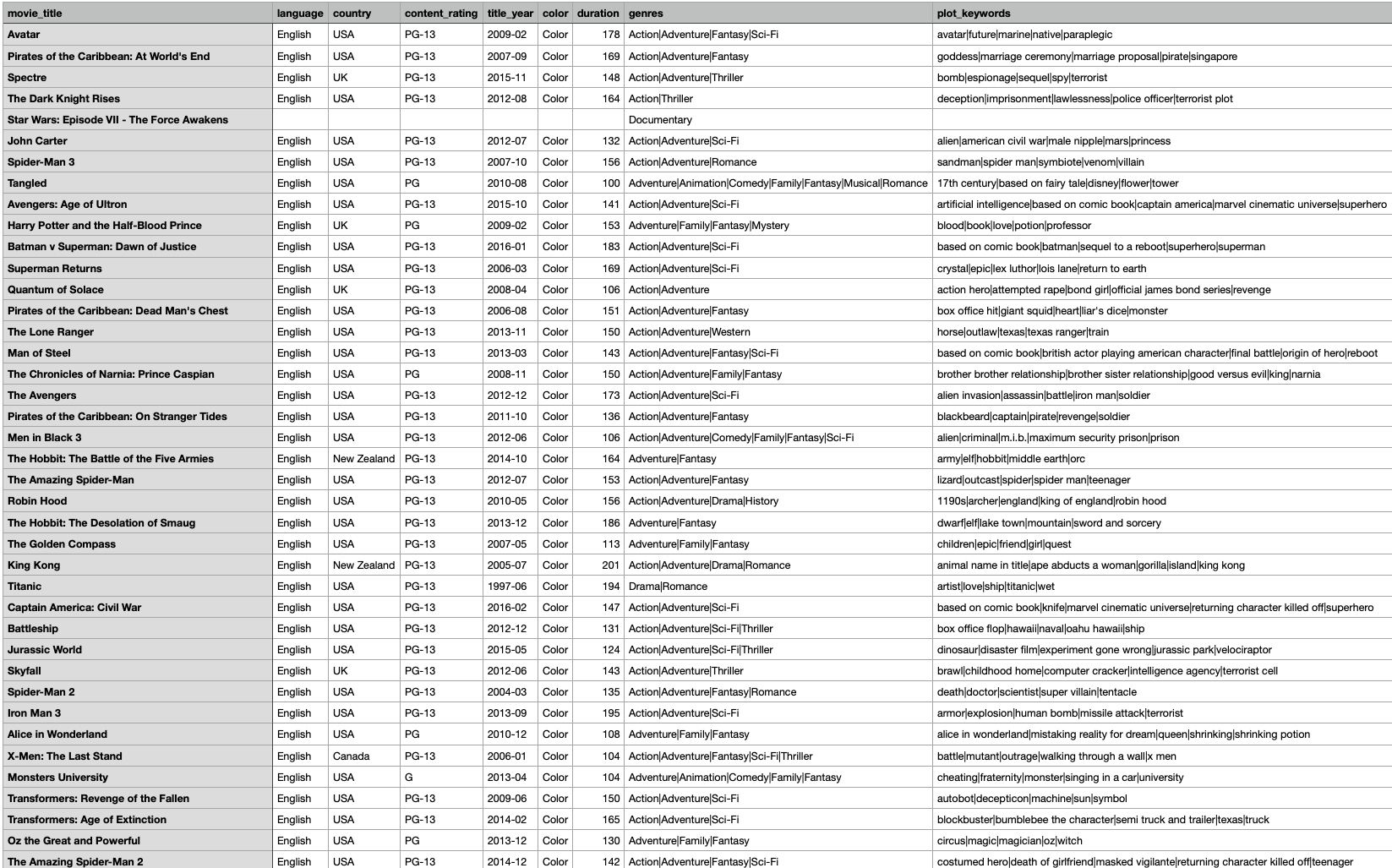
也就是说，我们大部分时候要处理的数据，基本上都一组二维数据。例如，我们今天最后案例要用到的一个电影数据(部分)，如图：

20231226133842

这里面，我们就将数据通过行列来展示和定位。

了解了这一点之后，我们来开始学习 pandas。

Pandas 简介

在之前的介绍中，我们发现很多的操作似乎都似曾相识，在 NumPy 中我们好像都接触过。

有这种感觉很正常，Pandas 本身就是基于 NumPy 的一种工具，该⼯具是为了解决数据分析任务⽽创建的。Pandas 纳⼊了⼤量库和⼀些标准的数据模型，提供了⾼效地操作⼤型数据集所需的⼯具。pandas 提供了⼤量能使我们快速便捷地处理数据的函数和⽅法。

Series 对象

Pandas 基于两种数据类型：series与dataframe。

Series是 Pandas 中最基本的对象，Series 类似⼀种⼀维数组。事实上，Series 基本上就是基于 NumPy 的数组对象来的。和 NumPy 的数组不同，Series 能为数据⾃定义标签，也就是索引（index），然后通过索引来访问数组中的数据。

Dataframe是⼀个⼆维的表结构。Pandas 的 dataframe 可以存储许多种不同的数据类型，并且每⼀个坐标轴都有⾃⼰的标签。你可以把它想象成⼀个 series 的字典项。

在开始基于代码进行学习之前，我们需要应用一些必要项。

import numpy as np
import pandas as pd
from pandas import Series
from pandas import DataFrame as df

现在我们来看看 Series 的一些基本操作：

创建 Series 对象并省略索引

index 参数是可省略的，你可以选择不输⼊这个参数。如果不带 index 参数，Pandas 会⾃动⽤默认 index 进⾏索引，类似数组，索引值是 [0, ..., len(data) - 1]

sel = Series([1,2,3,4])
print(sel)

---
0    1
1    2
2    3
3    4
dtype: int64

我们之前在 NumPy 中学习了 dtype, 以及它的相关数据类型。所以现在的dtype: int64我们应该能理解是什么意思了。

我们看打印的结果，在1,2,3,4前面，是 Series 默认生成的索引值。

通常我们会⾃⼰创建索引

sel = Series(data=[1,2,3,4], index= list('abcd'))
print(sel)

---
a    1
b    2
c    3
d    4
dtype: int64

这个时候，我们可以对这个 Series 对象操作分别获取内容和索引：

print(f'values: {sel.values}')
print(sel.index)

---
values: [1 2 3 4]
Index(['a', 'b', 'c', 'd'], dtype='object')

又或者，我们可以直接获取健值对（索引和值对）。

print(list(sel.iteritems()))

---
[('a', 1), ('b', 2), ('c', 3), ('d', 4)]

那么这种健值对的形式让你想到了什么？是字典对吧？

我们完全可以将字典转为 Series:

dict={"red":100,"black":400,"green":300,"pink":900}
se3=Series(dict) 
print(se3)

---
red      100
black    400
green    300
pink     900
dtype: int64

Series 数据获取

在 Series 拿到数据转为 Series 对象之后，诺大的数据中，我们如何定位并获取到我们想要的内容呢？

Series 在获取数据上，支持位置、标签、获取不连续数据，使用切片等方式。我们一个个的看一下：

Series 对象同时⽀持位置和标签两种⽅式获取数据

print('索引下标',sel['c'])
print('位置下标',sel[2])

---
索引下标 3
位置下标 3

获取不连续的数据

print('位置切⽚\n',sel[1:3])# 左包含右不包含
print('\n 索引切⽚\n',sel['b':'d'])# 左右都包含

---
位置切⽚
b    2
c    3
dtype: int64

索引切⽚
b    2
c    3
d    4
dtype: int64

我们看到结果，发现两组数据数量不对，但是其实我们获取的位置都是一样的。这是因为，位置切片的方式会是「左包含右不包含」的，而索引切片则是「左右都包含」。

重新赋值索引的值

除了获取数据之外，我们还可以对数据进行重新索引。其实在之前我们将索引的时候，第二种自己赋值的方式实际上就是一个重新赋值了，将自己定义的值替换了默认值。这里让我们再来看一下：

sel.index = list('dcba')
print(sel)

---
d    1
c    2
b    3
a    4
dtype: int64

还有一种重新索引的方法reindex，这会返回一个新的 Series。调用reindex将会重新排序，缺失值这会用NaN填补。

print(sel.reindex(['b','a','c','d','e']))

---
b    3.0
a    4.0
c    2.0
d    1.0
e    NaN
dtype: float64

在重新索引的时候，我们特意多增加了一个索引。在最后一位没有数据的情况下，缺失值被NaN填补上了。

丢弃指定轴上的项

sel = pd.Series(range(10, 15))
print(sel)
print(sel.drop([2,3]))

---
0    10
1    11
2    12
3    13
4    14
dtype: int64
0    10
1    11
4    14
dtype: int64

使用drop，会丢弃掉轴上的项，例子中，我们将 2，3 进行了丢弃。

Series 进⾏算术运算操作

对 Series 的算术运算都是基于 index 进⾏的。我们可以⽤加减乘除（+ - * /）这样的运算符对两个 Series 进⾏运算，Pandas 将会根据索引 index，对响应的数据进⾏计算，结果将会以浮点数的形式存储，以避免丢失精度。如果 Pandas 在两个 Series ⾥找不到相同的 index，对应的位置就返回⼀个空值 NaN。

# Series 算数运算
series1 = pd.Series([1,2,3,4],['London','HongKong','Humbai','lagos'])
series2 = pd.Series([1,3,6,4],['London','Accra','lagos','Delhi'])

print('series1-series2:')
print(series1-series2) 
print('\nseries1+series2:')
print(series1+series2) 
print('\nseries1*series2:')
print(series1*series2)

---
series1-series2:
Accra       NaN
Delhi       NaN
HongKong    NaN
Humbai      NaN
London      0.0
lagos      -2.0
dtype: float64

series1+series2:
Accra        NaN
Delhi        NaN
HongKong     NaN
Humbai       NaN
London       2.0
lagos       10.0
dtype: float64

series1*series2:
Accra        NaN
Delhi        NaN
HongKong     NaN
Humbai       NaN
London       1.0
lagos       24.0
dtype: float64

除此之外，Series 的算术运算操作同样也支持 NumPy 的数组运算

sel = Series(data = [1,6,3,5], index = list('abcd'))
print(sel[sel>3]) # 布尔数组过滤
print(sel*2) # 标量乘法
print(np.square(sel)) # 可以直接加⼊到 numpy 的数学函数

---
b    6
d    5
dtype: int64
a     2
b    12
c     6
d    10
dtype: int64
a     1
b    36
c     9
d    25
dtype: int64

DataFrame

DataFrame（数据表）是⼀种 2 维数据结构，数据以表格的形式存储，分成若⼲⾏和列。通过 DataFrame，你能很⽅便地处理数据。常见的操作⽐如选取、替换⾏或列的数据，还能重组数据表、修改索引、多重筛选等。我们基本上可以把 DataFrame 理解成⼀组采⽤同样索引的 Series 的集合。调⽤ DataFrame()可以将多种格式的数据转换为 DataFrame 对象，它的的三个参数data、index和columns 分别为数据、⾏索引和列索引。

DataFrame 的创建

我们可以使用二维数组

df1 = df(np.random.randint(0,10,(4,4)),index=[1,2,3,4],columns=['a','b','c','d']) 
print(df1)

---
   a  b  c  d
1  9  6  3  0
2  6  2  7  0
3  3  1  6  5
4  6  6  7  1

也可以使用字典创建

行索引由 index 决定，列索引由字典的键决定

dict={'Province': ['Guangdong', 'Beijing', 'Qinghai','Fujian'],'pop': [1.3, 2.5, 1.1, 0.7], 'year': [2022, 2022, 2022, 2022]}
df2= df(dict,index=[1,2,3,4]) 
print(df2)

---
    Province  pop  year
1  Guangdong  1.3  2022
2    Beijing  2.5  2022
3    Qinghai  1.1  2022
4     Fujian  0.7  2022

使用from_dict

dict2={"a":[1,2,3],"b":[4,5,6]}
df6=df.from_dict(dict2) 
print(df6)

---
   a  b
0  1  4
1  2  5
2  3  6

索引相同的情况下，相同索引的值会相对应，缺少的值会添加NaN

data = {
 'Name':pd.Series(['zs','ls','we'],index=['a','b','c']),
 'Age':pd.Series(['10','20','30','40'],index=['a','b','c','d']),
 'country':pd.Series(['中国','⽇本','韩国'],index=['a','c','b'])
}
df = pd.DataFrame(data)
print(df)

---
  Name Age country
a   zs  10      中国
b   ls  20      韩国
c   we  30      ⽇本
d  NaN  40     NaN

看了那么多 DataFrame 的转换方式，那我们如何将数据转为字典呢？DataFrame 有一个内置方法to_dict()能将 DataFrame 对象转换为字典：

dict = df.to_dict()
print(dict)

---
{'Name': {'a': 'zs', 'b': 'ls', 'c': 'we', 'd': nan}, 'Age': {'a': '10', 'b': '20', 'c': '30', 'd': '40'}, 'country': {'a': '中国', 'b': '韩国', 'c': '⽇本', 'd': nan}}

DataFrame 对象常⽤属性

让我们先来生成一组数据备用：

df_dict = {
'name':['James','Curry','Iversion'],
'age':['18','20','19'],
 'national':['us','China','us'] }
df = pd.DataFrame(data=df_dict,index=['0','1','2'])
print(df)

---
       name age national
0     James  18       us
1     Curry  20    China
2  Iversion  19       us

获取⾏数和列数

print(df.shape)

---
(3,3)

获取⾏索引

print(df.index.tolist())

---
['0', '1', '2']

获取列索引

print(df.columns.tolist())

---
['name', 'age', 'national']

获取数据的类型

print(df.dtypes)

---
name        object
age         object
national    object
dtype: object

获取数据的维度

print(df.ndim)

---
2

values 属性也会以⼆维 ndarray 的形式返回 DataFrame 的数据

print(df.values)

---
[['James' '18' 'us']
 ['Curry' '20' 'China']
 ['Iversion' '19' 'us']]

展示 df 的概览

print(df.info())

---
<class 'pandas.core.frame.DataFrame'>
Index: 3 entries, 0 to 2
Data columns (total 3 columns):
 #   Column    Non-Null Count  Dtype 
---  ------    --------------  ----- 
 0   name      3 non-null      object
 1   age       3 non-null      object
 2   national  3 non-null      object
dtypes: object(3)
memory usage: 96.0+ bytes
None

显示头⼏⾏,默认显示 5⾏

print(df.head(2))

---
    name age national
0  James  18       us
1  Curry  20    China

显示后⼏⾏

print(df.tail(1))

---
       name age national
2  Iversion  19       us

获取 DataFrame 的列

print(df['name'])

---
0       James
1       Curry
2    Iversion
Name: name, dtype: object

因为我们只获取⼀列，所以返回的就是⼀个 Series

print(type(df['name']))

---
<class 'pandas.core.series.Series'>

如果获取多个列，那返回的就是⼀个 DataFrame 类型：

print(df[['name','age']])
print(type(df[['name','age']]))

---
       name age
0     James  18
1     Curry  20
2  Iversion  19
<class 'pandas.core.frame.DataFrame'>

获取一行

print(df[0:1])

---
    name age national
0  James  18       us

去多⾏

print(df[1:3])

---
       name age national
1     Curry  20    China
2  Iversion  19       us

取多⾏⾥⾯的某⼀列（不能进⾏多⾏多列的选择）

print(df[1:3][['name','age']])

---
       name age
1     Curry  20
2  Iversion  19

⚠️ 注意：df[]只能进⾏⾏选择，或列选择，不能同时多⾏多列选择。比如在 NumPy 中的data[:,1:3]这种是不行的。当然，并不是没有办法获取，我们接着往下看:

df.loc通过标签索引⾏数据;df.iloc通过位置获取⾏数据

获取某⼀⾏某⼀列的数据

print(df.loc['0','name'])

---
James

⼀⾏所有列

print(df.loc['0',:])

---
name        James
age            18
national       us
Name: 0, dtype: object

某⼀⾏多列的数据

print(df.loc['0',['name','age']])

---
name    James
age        18
Name: 0, dtype: object

选择间隔的多⾏多列

print(df.loc[['0','2'],['name','national']]) 

---
       name national
0     James       us
2  Iversion       us

选择连续的多⾏和间隔的多列

print(df.loc['0':'2',['name','national']])

---
       name national
0     James       us
1     Curry    China
2  Iversion       us

取⼀⾏

print(df.iloc[1])

---
name        Curry
age            20
national    China
Name: 1, dtype: object

取连续多⾏

print(df.iloc[0:2])

---
    name age national
0  James  18       us
1  Curry  20    China

取间断的多⾏

print(df.iloc[[0,2],:])

---
       name age national
0     James  18       us
2  Iversion  19       us

取某⼀列

print(df.iloc[:,1])

---
0    18
1    20
2    19
Name: age, dtype: object

某⼀个值

print(df.iloc[1,0])

---
Curry

修改值

df.iloc[0,0]='panda'
print(df)

---
       name age national
0     panda  18       us
1     Curry  20    China
2  Iversion  19       us

dataframe 中的排序⽅法

df = df.sort_values(by='age', ascending*=False) 
print(df)

---
       name age national
1     Curry  20    China
2  Iversion  19       us
0     panda  18       us

ascending=False是降序排列，默认为True，也就是升序。

dataframe修改index、columns

一样，让我们先创建一组新的数据供我们使用：

df1 = pd.DataFrame(np.arange(9).reshape(3, 3), index = ['bj', 'sh', 'gz'], columns=['a', 'b', 'c'])
print(df1)

---
    a  b  c
bj  0  1  2
sh  3  4  5
gz  6  7  8

修改 df1 的 index

df1.index可以打印出 df1 的索引值，同时也可以为其赋值。

print(df1.index) # 可以打印出 print 的值，同时也可以为其赋值
df1.index = ['beijing', 'shanghai', 'guangzhou']
print(df1)

---
Index(['bj', 'sh', 'gz'], dtype='object')
           a  b  c
beijing    0  1  2
shanghai   3  4  5
guangzhou  6  7  8

⾃定义 map 函数（x 是原有的⾏列值）

# ⾃定义 map 函数（x 是原有的⾏列值） 
def test_map(x):
    return x+'_ABC'
print(df1.rename(index=test_map, columns=test_map, inplace=True))
print(df1)

---
None
               a_ABC  b_ABC  c_ABC
beijing_ABC        0      1      2
shanghai_ABC       3      4      5
guangzhou_ABC      6      7      8

其中的inplace传入一个布尔值，默认为 False。指定是否返回新的 DataFrame。如果为 True，则在原 df 上修改，返回值为 None。

rename 可以传⼊字典，为某个 index 单独修改名称

df3 = df1.rename(index={'beijing_ABC':'beijing'}, columns = {'a_ABC':'aa'})
print(df3)

---
               aa  b_ABC  c_ABC
beijing         0      1      2
shanghai_ABC    3      4      5
guangzhou_ABC   6      7      8

列转化为索引

df1=pd.DataFrame({'X':range(5),'Y':range(5),'S':list("abcde"),'Z': [1,1,2,2,2]})
print(df1)

---
   X  Y  S  Z
0  0  0  a  1
1  1  1  b  1
2  2  2  c  2
3  3  3  d  2
4  4  4  e  2

指定⼀列为索引 (drop=False 指定同时保留作为索引的列)

result = df1.set_index('S',drop=False)
result.index.name=None
print(result)

---
   X  Y  S  Z
a  0  0  a  1
b  1  1  b  1
c  2  2  c  2
d  3  3  d  2
e  4  4  e  2

⾏转为列索引

result = df1.set_axis(df1.iloc[0],axis=1,inplace=False)
result.columns.name=None
print(result)

---
   0  0  a  1
0  0  0  a  1
1  1  1  b  1
2  2  2  c  2
3  3  3  d  2
4  4  4  e  2

添加数据

先增加一组数据：

df1 = pd.DataFrame([['Snow','M',22],['Tyrion','M',32],['Sansa','F',18], ['Arya','F',14]],columns=['name','gender','age'])
print(df1)

---
     name gender  age
0    Snow      M   22
1  Tyrion      M   32
2   Sansa      F   18
3    Arya      F   14

在数据框最后加上 score⼀列，注意增加列的元素个数要跟原数据列的个数⼀样。

df1['score']=[80,98,67,90] 
print(df1)

---
     name gender  age  score
0    Snow      M   22     80
1  Tyrion      M   32     98
2   Sansa      F   18     67
3    Arya      F   14     90

在具体某个位置插⼊⼀列可以⽤insert的⽅法, 语法格式：列表.insert(index, obj)

index --->对象 obj 需要插⼊的索引位置。

obj---> 要插⼊列表中的对象（列名）

将数据框的列名全部提取出来存放在列表⾥

col_name=df1.columns.tolist() 
print(col_name)

---
['name', 'gender', 'age', 'score']

在列索引为 2 的位置插⼊⼀列,列名为:city

col_name.insert(2,'city')
print(col_name)

---
['name', 'gender', 'city', 'age', 'score']

刚插⼊时不会有值，整列都是 NaN,我们使用DataFrame.reindex()对原⾏/列索引重新构建索引值

df1=df1.reindex(columns=col_name)
print(df1)

---
     name gender  city  age  score
0    Snow      M   NaN   22     80
1  Tyrion      M   NaN   32     98
2   Sansa      F   NaN   18     67
3    Arya      F   NaN   14     90

给 city 列赋值

df1['city']=['北京京','⼭⻄西','湖北北','澳⻔门'] 
print(df1)

---
     name gender city  age  score
0    Snow      M  北京京   22     80
1  Tyrion      M  ⼭⻄西   32     98
2   Sansa      F  湖北北   18     67
3    Arya      F  澳⻔门   14     90

df 中的insert是插⼊⼀列。语法和关键参数为：

df.insert(iloc,column,value)

iloc:要插⼊的位置

colunm:列名

value:值

刚才我们插入city列的时候省略了value,所以新建列值全部为NaN，这次我们加上再看：

df1.insert(2,'score2',[80,98,67,90]) 
print(df1)

---
     name gender  score2 city  age  score
0    Snow      M      80  北京京   22     80
1  Tyrion      M      98  ⼭⻄西   32     98
2   Sansa      F      67  湖北北   18     67
3    Arya      F      90  澳⻔门   14     90

插⼊⼀⾏

# 插⼊⼀⾏
row=['111','222','333','444','555','666'] 
df1.iloc[1]=row
print(df1)

---
    name gender score2 city  age score
0   Snow      M     80  北京京   22    80
1    111    222    333  444  555   666
2  Sansa      F     67  湖北北   18    67
3   Arya      F     90  澳⻔门   14    90

插入行的时候，列个数必须对应才可以，否则会报错。

目前这组数据已经被我们玩乱了，我们再重新生成一组数据来看后面的：

df1 = pd.DataFrame([['Snow','M',22],['Tyrion','M',32],['Sansa','F',18],['Arya','F',14]],columns=['name','gender','age'])
print(df1)

---
     name gender  age
0    Snow      M   22
1  Tyrion      M   32
2   Sansa      F   18
3    Arya      F   14

再继续创建一组数据，我们将尝试将两组数据进行合并, 新创建的这组数据⽤来增加进数据框的最后⼀⾏。

new=pd.DataFrame({'name':'lisa','gender':'F','age':19},index=[0])
print(new)

---
   name gender  age
0  lisa      F   19

在原数据框 df1 最后⼀⾏新增⼀⾏，⽤append⽅法

df1=df1.append(new,ignore_index=True) 
print(df1)

---
     name gender  age
0    Snow      M   22
1  Tyrion      M   32
2   Sansa      F   18
3    Arya      F   14
4    lisa      F   19

ignore_index=False,表示不按原来的索引，从 0 开始⾃动递增。

objs:合并对象

axis:合并⽅式，默认 0 表示按列合并，1 表示按⾏合并

ignore_index:是否忽略索引

df1 = pd.DataFrame(np.arange(6).reshape(3,2),columns=['four','five'])
df2 = pd.DataFrame(np.arange(6).reshape(2,3),columns=['one','two','three'])
print(df1)
print(df2)

---
   four  five
0     0     1
1     2     3
2     4     5
   one  two  three
0    0    1      2
1    3    4      5

按行合并

result = pd.concat([df1,df2],axis=1)
print(result)

---
   four  five  one  two  three
0     0     1  0.0  1.0    2.0
1     2     3  3.0  4.0    5.0
2     4     5  NaN  NaN    NaN

按列合并

   four  five  one  two  three
0   0.0   1.0  NaN  NaN    NaN
1   2.0   3.0  NaN  NaN    NaN
2   4.0   5.0  NaN  NaN    NaN
3   NaN   NaN  0.0  1.0    2.0
4   NaN   NaN  3.0  4.0    5.0

看结果我们能看出来，在合并的时候，如果对应不到值，那么就会默认添加NaN值。

DataFrame 的删除

df2 = pd.DataFrame(np.arange(9).reshape(3,3),columns=['one','two','three'])
print(df2)
df3=df2.drop(['one'],axis=1, inplace=True)
print(df2)
print(df3)

---
   one  two  three
0    0    1      2
1    3    4      5
2    6    7      8
   two  three
0    1      2
1    4      5
2    7      8
None

lables：要删除数据的标签

axis：0 表示删除⾏，1 表示删除列，默认 0

inplace:是否在当前 df 中执⾏此操作

最后的返回值为None，原因是我们设置inplace为True，在当前df中执行操作。如果我们将其设置为False，则会将操作后的值进行返回，生成一个新的对象。

df3=df2.drop([0,1],axis=0, inplace=False)
print(df2)
print(df3)

---
   one  two  three
0    0    1      2
1    3    4      5
2    6    7      8
   one  two  three
2    6    7      8

数据处理

在我们查看完 DataFrame 的基础操作之后，我们现在来正式开始数据处理。

我们可以通过通过dropna()滤除缺失数据，先让我们创建一组数据：

se=pd.Series([4,NaN,8,NaN,5]) 
print(se)

---
0    4.0
1    NaN
2    8.0
3    NaN
4    5.0
dtype: float64

尝试清除缺失数据，也就是NaN值：

print(se.dropna())

---
0    4.0
2    8.0
4    5.0
dtype: float64

在清除数据之前，我们有两个方法可以判断当前数据中是否有缺失数据，不过这两个方法的判断方式是相反的，一个是判断不是缺失数据，一个判断是缺失数据：

print(se.notnull())
print(se.isnull())

---
0     True
1    False
2     True
3    False
4     True
dtype: bool
0    False
1     True
2    False
3     True
4    False
dtype: bool

那既然有方法可以进行判断当前数据是否为缺失数据，那么我们用之前的方法与其配合，一样可以做滤除操作：

print(se[se.notnull()])

---
0    4.0
2    8.0
4    5.0
dtype: float64

当然，除了 Series 对象之外，我们还需要进行处理 DataFrame 对象

df1=pd.DataFrame([[1,2,3],[NaN,NaN,2],[NaN,NaN,NaN],[8,8,NaN]]) 
print(df1)

---
     0    1    2
0  1.0  2.0  3.0
1  NaN  NaN  2.0
2  NaN  NaN  NaN
3  8.0  8.0  NaN

默认滤除所有包含NaN：

print(df1.dropna())

---
     0    1    2
0  1.0  2.0  3.0

传⼊how=‘all’滤除全为NaN的⾏：

print(df1.dropna(how='all')) 

---
     0    1    2
0  1.0  2.0  3.0
1  NaN  NaN  2.0
3  8.0  8.0  NaN

可以看到，除了下标为2的那一行之外，其余含NaN值的行都被保留了。

之前操作最后只留下一行，原因是how的默认值为how='any'。只要是nan就删除

传⼊axis=1 滤除列：

print(df1.dropna(axis=1,how="all"))

---
     0    1    2
0  1.0  2.0  3.0
1  NaN  NaN  2.0
2  NaN  NaN  NaN
3  8.0  8.0  NaN

为什么没有变化？按列来查看，没有一列是全是NaN值的。

除了how值外，我们还可以可以使用thresh来精准操作，它可以传入一个数值n，会保留至少n个非NaN数据的行或列：

print(df1.dropna(thresh=2))

---
     0    1    2
0  1.0  2.0  3.0
3  8.0  8.0  NaN

仅有一个非NaN的行和全部为NaN的行就都被滤除了。

那NaN是不是就只能被删除了呢？并不是，还记得我们之前操作的时候我提到过，我们大多数遇到NaN值的时候，基本都是用平均值来进行填充，这是一个惯例操作。

那么，我们来看看如何填充缺失数据

df1=pd.DataFrame([[1,2,3],[NaN,NaN,2],[NaN,NaN,NaN],[8,8,NaN]]) 
print(df1)

---
     0    1    2
0  1.0  2.0  3.0
1  NaN  NaN  2.0
2  NaN  NaN  NaN
3  8.0  8.0  NaN

⽤常数填充fillna

print(df1.fillna(0))

---
     0    1    2
0  1.0  2.0  3.0
1  0.0  0.0  2.0
2  0.0  0.0  0.0
3  8.0  8.0  0.0

传⼊inplace=True直接修改原对象：

df1.fillna(0,inplace=True) 
print(df1)

---
     0    1    2
0  1.0  2.0  3.0
1  0.0  0.0  2.0
2  0.0  0.0  0.0
3  8.0  8.0  0.0

通过字典填充不同的常数

print(df1.fillna({0:10,1:20,2:30}))

---
      0     1     2
0   1.0   2.0   3.0
1  10.0  20.0   2.0
2  10.0  20.0  30.0
3   8.0   8.0  30.0

还有我们之前提到过的，填充平均值：

print(df1.fillna(df1.mean()))

---
     0    1    2
0  1.0  2.0  3.0
1  4.5  5.0  2.0
2  4.5  5.0  2.5
3  8.0  8.0  2.5

当然，我们可以只填充某一列

print(df1.iloc[:,1].fillna(5,inplace = True)) 
print(df1)

---
None
     0    1    2
0  1.0  2.0  3.0
1  NaN  5.0  2.0
2  NaN  5.0  NaN
3  8.0  8.0  NaN

传⼊method=” “会改变插值⽅式，先来一组数据，并在其中加上NaN值

df2=pd.DataFrame(np.random.randint(0,10,(5,5))) 
df2.iloc[1:4,3]=NaN
df2.iloc[2:4,4]=NaN
print(df2)

---
   0  1  2    3    4
0  3  5  9  9.0  3.0
1  0  1  2  NaN  8.0
2  6  5  8  NaN  NaN
3  5  6  5  NaN  NaN
4  5  3  5  8.0  2.0

现在，我们用前面的值来填充， method ='ffill'

print(df2.fillna(method='ffill'))

---
   0  1  2    3    4
0  3  5  9  9.0  3.0
1  0  1  2  9.0  8.0
2  6  5  8  9.0  8.0
3  5  6  5  9.0  8.0
4  5  3  5  8.0  2.0

用后面的值来填充method='bfill':

print(df2.fillna(method='bfill',limit=1))

---
   0  1  2    3    4
0  7  1  8  0.0  0.0
1  6  8  4  NaN  5.0
2  6  2  5  NaN  NaN
3  4  8  0  1.0  3.0
4  8  0  2  1.0  3.0

以上代码中，我们还传入了limit，用于限制填充行数。

当我们传入axis的时候，会修改填充方向：

print(df2.fillna(method="ffill",limit=1,axis=1))

---
     0    1    2    3    4
0  0.0  8.0  9.0  4.0  7.0
1  2.0  8.0  0.0  0.0  9.0
2  1.0  8.0  5.0  5.0  NaN
3  0.0  0.0  3.0  3.0  NaN
4  2.0  9.0  4.0  6.0  3.0

接着，我们再来看看如何移除重复数据，俗称「去重」：

DataFrame 中经常会出现重复⾏，利⽤duplicated()函数返回每⼀⾏判断是否重复的结果（重复则为 True)

df1=pd.DataFrame({'A':[1,1,1,2,2,3,1],'B':list("aabbbca")})
print(df1)
print(df1.duplicated())

---
   A  B
0  1  a
1  1  a
2  1  b
3  2  b
4  2  b
5  3  c
6  1  a

0    False
1     True
2    False
3    False
4     True
5    False
6     True
dtype: bool

去除全部的重复⾏

print(df1.drop_duplicates())

---
   A  B
0  1  a
2  1  b
3  2  b
5  3  c

指定列去除重复行

print(df1.drop_duplicates(['A']))

---
   A  B
0  1  a
3  2  b
5  3  c

保留重复⾏中的最后⼀⾏

df1=pd.DataFrame({'A':[1,1,1,2,2,3,1],'B':list("aabbbca")})
print(df1.drop_duplicates(['A'],keep='last'))

---
   A  B
4  2  b
5  3  c
6  1  a

去除重复的同时改变 DataFrame 对象

df1.drop_duplicates(['A','B'],inplace=True) 
print(df1)

---
   A  B
0  1  a
2  1  b
3  2  b
5  3  c

数据合并

我们平时会与拿到的数据可能存储在不同的数据表中，这需要我们对数据进行合并，然后再进行操作。

使⽤join合并，着重关注的是⾏的合并。

简单合并（默认是 left 左连接,以左侧df3为基础）

df3=pd.DataFrame({'Red':[1,3,5],'Green':[5,0,3]},index=list('abc'))
df4=pd.DataFrame({'Blue':[1,9,8],'Yellow':[6,6,7]},index=list('cde')) 
print(df3)
print(df4)
df3.join(df4,how='left')

---
   Red  Green
a    1      5
b    3      0
c    5      3
   Blue  Yellow
c     1       6
d     9       6
e     8       7


	Red	Green	Blue	Yellow
a	1		5			NaN		NaN
b	3		0			NaN		NaN
c	5		3			1.0		6.0

右链接

df3.join(df4,how='outer')

---
	Red	Green	Blue	Yellow
a	1.0	5.0		NaN		NaN
b	3.0	0.0		NaN		NaN
c	5.0	3.0		1.0		6.0
d	NaN	NaN		9.0		6.0
e	NaN	NaN		8.0		7.0

合并多个 DataFrame 对象

df5=pd.DataFrame({'Brown':[3,4,5],'White':[1,1,2]},index=list('aed')) 
df3.join([df4,df5])

---

	Red	Green	Blue	Yellow	Brown	White
a	1.0	5.0		NaN		NaN			3.0		1.0
b	3.0	0.0		NaN		NaN			NaN		NaN
c	5.0	3.0		1.0		6.0			NaN		NaN

使⽤merge，着重关注的是列的合并。

我们先来构建两组数据：

df1=pd.DataFrame({'名字':list('ABCDE'),'性别':['男','⼥','男','男','⼥'],'职称': ['副教授','讲师','助教','教授','助教']},index=range(1001,1006))
df1.columns.name='学院⽼师'
df1.index.name='编号'
df1

---
学院⽼师	名字	性别	职称
编号			
1001		A			男		副教授
1002		B			⼥		讲师
1003		C			男		助教
1004		D			男		教授
1005		E			⼥		助教

df2=pd.DataFrame({'名字':list('ABDAX'),'课程':['C++','计算机导论','汇编','数据结构','马克思原理'],'职称':['副教授','讲师','教授','副教授','讲师']},index= [1001,1002,1004,1001,3001])
df2.columns.name='课程'
df2.index.name='编号'
print(df2)

---
课程	名字	课程				职称
编号			
1001	A		C++				副教授
1002	B		计算机导论		讲师
1004	D		汇编				教授
1001	A		数据结构		副教授
3001	X		马克思原理	讲师

默认下是根据左右对象中出现同名的列作为连接的键，且连接⽅式是how=’inner’

print(pd.merge(df1,df2)) # 返回匹配的

---
  名字 性别   职称     课程
0  A  男  副教授    C++
1  A  男  副教授   数据结构
2  B  ⼥   讲师  计算机导论
3  D  男   教授     汇编

指定列名合并

pd.merge(df1,df2,on='名字',suffixes=['_1','_2']) # 返回匹配的

---

	名字	性别	职称_1	课程		职称_2
0	A			男		副教授		C++			副教授
1	A			男		副教授		数据结构	副教授
2	B			⼥		讲师		计算机导论	讲师
3	D			男		教授		汇编			教授

连接⽅式，根据左侧为准

pd.merge(df1,df2,how='left')

---
	名字	性别	职称	课程
0	A			男	副教授	C++
1	A			男	副教授	数据结构
2	B			⼥	讲师	计算机导论
3	C			男	助教	NaN
4	D			男	教授	汇编
5	E			⼥	助教	NaN

根据右侧为准

pd.merge(df1,df2,how='right')

---
	名字	性别	职称	课程
0	A		男	副教授	C++
1	B		⼥	讲师	计算机导论
2	D		男	教授	汇编
3	A		男	副教授	数据结构
4	X		NaN	讲师	马克思原理

所有的数据

pd.merge(df1,df2,how='outer')

---

名字	性别	职称	课程
0		A	男	副教授	C++
1		A	男	副教授	数据结构
2		B	⼥	讲师	计算机导论
3		C	男	助教	NaN
4		D	男	教授	汇编
5		E	⼥	助教	NaN
6		X	NaN	讲师	马克思原理

根据多个键进⾏连接

pd.merge(df1,df2,*on*=['职称','名字'])

---
	名字	性别	职称	课程
0	A			男	副教授	C++
1	A			男	副教授	数据结构
2	B			⼥	讲师	计算机导论
3	D			男	教授	汇编

除此之外，我们还有一种轴向连接的方式：Concat

Series 对象的连接

s1=pd.Series([1,2],index=list('ab'))
s2=pd.Series([3,4,5],index=list('bde')) 
print(s1)
print(s2)
pd.concat([s1,s2])

---
a    1
b    2
dtype: int64
b    3
d    4
e    5
dtype: int64
a    1
b    2
b    3
d    4
e    5
dtype: int64

横向连接

pd.concat([s1,s2],*axis*=1)

---
	0		1
a	1.0	NaN
b	2.0	3.0
d	NaN	4.0
e	NaN	5.0

⽤内连接求交集(连接⽅式，共有’inner’,’left’,right’,’outer’)

pd.concat([s1,s2],axis=1,join='inner')

---
	0	1
b	2	3

创建层次化索引

pd.concat([s1,s2],keys=['A','B'])

---
A  a    1
   b    2
B  b    3
   d    4
   e    5
dtype: int64

当纵向连接时 keys 为列名

pd.concat([s1,s2],keys=['A','D'],axis=1)

----
	A		D
a	1.0	NaN
b	2.0	3.0
d	NaN	4.0
e	NaN	5.0

DataFrame 对象的连接

df3=pd.DataFrame({'Red':[1,3,5],'Green':[5,0,3]},index=list('abd')) 
df4=pd.DataFrame({'Blue':[1,9],'Yellow':[6,6]},index=list('ce'))
pd.concat([df3,df4])

---

	Red	Green	Blue	Yellow
a	1.0	5.0		NaN		NaN
b	3.0	0.0		NaN		NaN
d	5.0	3.0		NaN		NaN
c	NaN	NaN		1.0		6.0
e	NaN	NaN		9.0		6.0

⽤字典的⽅式连接同样可以创建层次化列索引

pd.concat({'A':df3,'B':df4},axis=1)

---
	A					B
	Red	Green	Blue	Yellow
a	1.0	5.0		NaN		NaN
b	3.0	0.0		NaN		NaN
d	5.0	3.0		NaN		NaN
c	NaN	NaN		1.0		6.0
e	NaN	NaN		9.0		6.0

多层索引（拓展）

创建多层索引

s = Series(np.random.randint(0,150,size=6),index=list('abcdef'))
print(s)

---
a     40
b    122
c     95
d     40
e     35
f     27
dtype: int64

s = Series(np.random.randint(0,150,size=6),
index=[['a','a','b','b','c','c'],['期中','期末','期中','期末','期中','期末']]) 
print(s)

---
a  期中    132
   期末    145
b  期中     33
   期末    149
c  期中     10
   期末    145
dtype: int64

DataFrame 也可以创建多层索引

# DataFrame 创建多层索引
df1 = df(np.random.randint(0,150,size=(6,4)),
         columns = ['zs','ls','ww','zl'],
         index =[['python','python','math','math','En','En'],['期中','期末','期中','期末','期中','期末']])
print(df1)

---
            zs   ls   ww   zl
python 期中  123    3   98   95
       期末    9   36   15  126
math   期中   86   86   73  115
       期末    3  130   52   89
En     期中   75   21   84   98
       期末   56   46  111  147

特定结构

class1=['python','python','math','math','En','En']
class2=['期中','期末','期中','期末','期中','期末']
m_index2=pd.MultiIndex.from_arrays([class1,class2])
df2=df(np.random.randint(0,150,(6,4)),index=m_index2) 
print(df2)

---
             0    1    2    3
python 期中   94   36    6   19
       期末   24   41  108  120
math   期中   79   69  144   32
       期末  138  100   42   38
En     期中  110   90  123   75
       期末   69   59   72  109

class1=['期中','期中','期中','期末','期末','期末']
class2=['python','math','En','python','math','En']
m_index2=pd.MultiIndex.from_arrays([class1,class2])
df2=df(np.random.randint(0,150,(6,4)),index=m_index2) 
print(df2)

---
             0   1    2    3
期中 python   96  15  135    5
   	math     66  78  143   93
   	En       70  27  120   63
期末 python  147  77   92   97
   	math    121  81  137  102
   	En       18  12  134  113

product 构造

class1=['python','math','En']
class2=['期中','期末']
m_index2=pd.MultiIndex.from_product([class1,class2])
df2=df(np.random.randint(0,150,(6,4)),index=m_index2) 
print(df2)

---
             0    1    2    3
python 期中   12   72  115   59
       期末   36   51   94  111
math   期中   44   14    9   61
       期末  115  121   65   93
En     期中   29   23   16   70
       期末   30   73   77   53

多层索引对象的索引

让我们先来看看 Series 的操作

s = Series(np.random.randint(0,150,size=6),
index=[['a','a','b','b','c','c'],['期中','期末','期中','期末','期中','期末']])
print(s)

---
a  期中     31
   期末      4
b  期中    101
   期末     95
c  期中     54
   期末    126
dtype: int64

取⼀个第⼀级索引

print(s['a'])

---
期中    31
期末     4
dtype: int64

取多个第⼀级索引

print(s[['a','b']])

---
a  期中     31
   期末      4
b  期中    101
   期末     95
dtype: int64

根据索引获取值

print(s['a','期末'])

---
4

loc⽅法取值

print(s.loc['a'])
print(s.loc[['a','b']]) 
print(s.loc['a','期末'])

---
期中    31
期末     4
dtype: int64
a  期中     31
   期末      4
b  期中    101
   期末     95
dtype: int64
4

iloc⽅法取值(iloc 计算的事最内层索引)

print(s.iloc[1])
print(s.iloc[1:4])

---
4
a  期末      4
b  期中    101
   期末     95
dtype: int64

然后再让我们来看看 DataFrame 的操作

# dataframe
class1=['python','math','En']
class2=['期中','期末']
m_index2=pd.MultiIndex.from_product([class1,class2])
df2=df(np.random.randint(0,150,(6,4)),index=m_index2) 
print(df2)

---
             0    1    2    3
python 期中   88   69   82   28
       期末  110   60  130  133
math   期中   64  103   24   49
       期末   23   41   10   61
En     期中  124  139   65  115
       期末  114   13  117   79

获取列

print(df2[0])

---
python  期中     88
        期末    110
math    期中     64
        期末     23
En      期中    124
        期末    114
Name: 0, dtype: int64

⼀级索引

print(df2.loc['python'])

---
      0   1    2    3
期中   88  69   82   28
期末  110  60  130  133

多个⼀级索引

print(df2.loc[['python','math']])

---
             0    1    2    3
python 期中   88   69   82   28
       期末  110   60  130  133
math   期中   64  103   24   49
       期末   23   41   10   61

取⼀⾏

print(df2.loc['python','期末'])

---
0    110
1     60
2    130
3    133
Name: (python, 期末), dtype: int64

取⼀值

print(df2.loc['python','期末'][0])

---
110

iloc 是只取最内层的索引的

print(df2.iloc[0])

---
0    88
1    69
2    82
3    28
Name: (python, 期中), dtype: int64

时间序列

⽣成⼀段时间范围

该函数主要⽤于⽣成⼀个固定频率的时间索引，在调⽤构造⽅法时，必须指定start、end、periods中的两个参数值，否则报错。

时间序列频率	解释
D	⽇历⽇的每天
B	⼯作⽇的每天
H	每⼩时
T 或 min	每分钟
S	每秒
L 或 ms	每毫秒
U	每微秒
M	⽇历⽇的⽉底⽇期
BM	⼯作⽇的⽉底⽇期
MS	⽇历⽇的⽉初⽇期
BMS	⼯作⽇的⽉初⽇期

date = pd.date_range(start='20190501',end='20190530')
print(date)

---
DatetimeIndex(['2023-05-01', '2023-05-02', '2023-05-03', '2023-05-04',
               '2023-05-05', '2023-05-06', '2023-05-07', '2023-05-08',
               '2023-05-09', '2023-05-10', '2023-05-11', '2023-05-12',
               '2023-05-13', '2023-05-14', '2023-05-15', '2023-05-16',
               '2023-05-17', '2023-05-18', '2023-05-19', '2023-05-20',
               '2023-05-21', '2023-05-22', '2023-05-23', '2023-05-24',
               '2023-05-25', '2023-05-26', '2023-05-27', '2023-05-28',
               '2023-05-29', '2023-05-30'],
              dtype='datetime64[ns]', freq='D')

req：⽇期偏移量，取值为 string, 默认为'D'，

periods：固定时期，取值为整数或 None

freq: 时间序列频率

date = pd.date_range(start='20230501',periods=10,freq='10D')
print(date)

---
DatetimeIndex(['2023-05-01', '2023-05-11', '2023-05-21', '2023-05-31',
               '2023-06-10', '2023-06-20', '2023-06-30', '2023-07-10',
               '2023-07-20', '2023-07-30'],
              dtype='datetime64[ns]', freq='10D')

根据closed参数选择是否包含开始和结束时间closed=None，left 包含开始时间，不包含结束时间， right 与之相反。

data_time =pd.date_range(start='2023-08-09',end='2023-08-14',closed='left') 
print(data_time)

---
DatetimeIndex(['2023-08-09', '2023-08-10', '2023-08-11', '2023-08-12',
               '2023-08-13'],
              dtype='datetime64[ns]', freq='D')

时间序列在 dataFrame 中的作⽤

可以将时间作为索引

index = pd.date_range(start='20230801',periods=10)
df = pd.Series(np.random.randint(0,10,size = 10),index=index) 
print(df)

---
2023-08-01    7
2023-08-02    2
2023-08-03    5
2023-08-04    5
2023-08-05    2
2023-08-06    0
2023-08-07    2
2023-08-08    3
2023-08-09    6
2023-08-10    5
Freq: D, dtype: int64

truncate这个函数将 before 指定⽇期之前的值全部过滤出去,after 指定⽇期之前的值全部过滤出去.

after = df.truncate(after='2023-08-8')
print(after)

---
2023-08-01    7
2023-08-02    2
2023-08-03    5
2023-08-04    5
2023-08-05    2
2023-08-06    0
2023-08-07    2
2023-08-08    3
Freq: D, dtype: int64

long_ts = pd.Series(np.random.randn(1000),index=pd.date_range('1/1/2021',periods=1000)) 
print(long_ts)

---
2021-01-01   -0.482811
...
2023-09-27   -0.108047
Freq: D, Length: 1000, dtype: float64

根据年份获取

result = long_ts['2022']
print(result)

---
2022-01-01   -0.600007
...
2022-12-31    0.097874
Freq: D, Length: 365, dtype: float64

年份和⽇期获取

result = long_ts['2023-07'] 
print(result)

---
2023-07-01   -1.797582
...
2023-07-31    0.687787
Freq: D, dtype: float64

使⽤切⽚

# 使⽤切⽚
result = long_ts['2023-05-01':'2023-05-06']
print(result)

---
2023-05-01   -2.338218
2023-05-02   -2.130780
2023-05-03    0.582920
2023-05-04   -0.182540
2023-05-05    0.127363
2023-05-06   -0.032844
Freq: D, dtype: float64

通过between_time()返回位于指定时间段的数据集

index=pd.date_range("2023-03-17","2023-03-30",freq="2H")
ts = pd.Series(np.random.randn(157),index=index) 
print(ts.between_time("7:00","17:00"))

---
2023-03-17 08:00:00   -0.532254
...
2023-03-29 16:00:00    0.437697
Length: 65, dtype: float64

这些操作也都适⽤于 dataframe

index=pd.date_range('1/1/2023',periods=100)
df = pd.DataFrame(np.random.randn(100,4),index=index) 
print(df.loc['2023-04'])

---
                   0         1         2         3
2023-04-01 -0.220090  0.335770 -0.086181 -0.046045
2023-04-02 -1.046423 -0.347116  0.367099 -0.979354
2023-04-03 -0.720944 -1.478932  0.220948  0.801831
2023-04-04  1.359946 -1.239004  0.309747 -0.047959
2023-04-05 -0.256502  2.224782  0.494740 -1.322490
2023-04-06  1.488119  0.244942  0.614101 -0.156201
2023-04-07 -1.815019 -1.935966  0.239024 -1.388502
2023-04-08  1.106623  1.148805  2.120405 -0.799290
2023-04-09 -1.902216  0.625965 -0.102506 -0.430550
2023-04-10 -0.876382 -2.034205 -0.060846  2.442651

移位⽇期

ts = pd.Series(np.random.randn(10),index=pd.date_range('1/1/2023',periods=10)) 
print(ts)

---
2023-01-01   -0.976958
2023-01-02   -0.487439
2023-01-03    0.143104
2023-01-04   -0.964236
2023-01-05    0.758326
2023-01-06   -1.650818
2023-01-07    0.709231
2023-01-08    0.198714
2023-01-09   -1.043443
2023-01-10    0.220834
Freq: D, dtype: float64

移动数据，索引不变，默认由NaN填充

periods: 移动的位数负数是向上移动

fill_value: 移动后填充数据

freq：⽇期偏移量

ts.shift(periods=2,fill_value=100, freq='D')

---
2023-01-03   -0.976958
2023-01-04   -0.487439
2023-01-05    0.143104
2023-01-06   -0.964236
2023-01-07    0.758326
2023-01-08   -1.650818
2023-01-09    0.709231
2023-01-10    0.198714
2023-01-11   -1.043443
2023-01-12    0.220834
Freq: D, dtype: float64

通过tshift()将索引移动指定的时间：

ts.tshift(2)

---
2023-01-03   -0.976958
2023-01-04   -0.487439
2023-01-05    0.143104
2023-01-06   -0.964236
2023-01-07    0.758326
2023-01-08   -1.650818
2023-01-09    0.709231
2023-01-10    0.198714
2023-01-11   -1.043443
2023-01-12    0.220834
Freq: D, dtype: float64

将时间戳转化成时间根式

pd.to_datetime(1688570740000,unit='ms')

---
Timestamp('2023-07-05 15:25:40')

utc 是协调世界时,时区是以 UTC 的偏移量的形式表示的,但是注意设置utc=True,是让 pandas 对象具有时区性质,对于⼀列进⾏转换的,会造成转换错误。

unit='ms'设置粒度是到毫秒级别的。

时区名字

import pytz
print(pytz.common_timezones)

---
['Africa/Abidjan', ..., 'US/Pacific', 'UTC']

pd.to_datetime(1688570740000,unit='ms').tz_localize('UTC').tz_convert('Asia/Shanghai')

---
Timestamp('2023-07-05 23:25:40+0800', tz='Asia/Shanghai')

一个处理的例子：

df = pd.DataFrame([1688570740000, 1688570800000, 1688570860000],columns = ['time_stamp'])
pd.to_datetime(df['time_stamp'],unit='ms').dt.tz_localize('UTC').dt.tz_convert ('Asia/Shanghai')

---
0   2023-07-05 23:25:40+08:00
1   2023-07-05 23:26:40+08:00
2   2023-07-05 23:27:40+08:00
Name: time_stamp, dtype: datetime64[ns, Asia/Shanghai]

先赋予标准时区,再转换到东⼋区。

处理中⽂

pd.to_datetime('2023 年 7⽉5⽇',format='%Y 年%m⽉%d⽇')

---
Timestamp('2023-07-05 00:00:00')

分组聚合

df=pd.DataFrame({
'name':['BOSS','Lilei','Lilei','Han','BOSS','BOSS','Han','BOSS'], 'Year':[2016,2016,2016,2016,2017,2017,2017,2017],
'Salary':[999999,20000,25000,3000,9999999,999999,3500,999999],
'Bonus':[100000,20000,20000,5000,200000,300000,3000,400000]
})
df

---

	name	Year	Salary	Bonus
0	BOSS	2016	999999	100000
1	Lilei	2016	20000		20000
2	Lilei	2016	25000		20000
3	Han		2016	3000		5000
4	BOSS	2017	9999999	200000
5	BOSS	2017	999999	300000
6	Han		2017	3500		3000
7	BOSS	2017	999999	400000

根据 name 这⼀列进⾏分组

group_by_name=df.groupby('name') 
print(type(group_by_name))

---
<class 'pandas.core.groupby.generic.DataFrameGroupBy'>

查看分组

print(group_by_name.groups) # 分组后的数量
print(group_by_name.count())

---
{'BOSS': [0, 4, 5, 7], 'Han': [3, 6], 'Lilei': [1, 2]}
       Year  Salary  Bonus
name                      
BOSS      4       4      4
Han       2       2      2
Lilei     2       2      2

查看分组的情况

for name,group in group_by_name: 
    print(name)
    
---
BOSS
Han
Lilei

组的名字

print(group) # 组具体内容

---
    name  Year  Salary  Bonus
1  Lilei  2016   20000  20000
2  Lilei  2016   25000  20000

可以选择分组

print(group_by_name.get_group('BOSS'))

---
   name  Year   Salary   Bonus
0  BOSS  2016   999999  100000
4  BOSS  2017  9999999  200000
5  BOSS  2017   999999  300000
7  BOSS  2017   999999  400000

按照某⼀列进⾏分组, 将 name 这⼀列作为分组的键，对 year 进⾏分组

group_by_name=df['Year'].groupby(df['name'])
print(group_by_name.count())

---
name
BOSS     4
Han      2
Lilei    2
Name: Year, dtype: int64

按照多列进⾏分组

group_by_name_year=df.groupby(['name','Year'])
for name,group in group_by_name_year: 
    print(name) # 组的名字
    print(group) # 组具体内容
    
---
('BOSS', 2016)
   name  Year  Salary   Bonus
0  BOSS  2016  999999  100000
('BOSS', 2017)
   name  Year   Salary   Bonus
4  BOSS  2017  9999999  200000
5  BOSS  2017   999999  300000
7  BOSS  2017   999999  400000
('Han', 2016)
  name  Year  Salary  Bonus
3  Han  2016    3000   5000
('Han', 2017)
  name  Year  Salary  Bonus
6  Han  2017    3500   3000
('Lilei', 2016)
    name  Year  Salary  Bonus
1  Lilei  2016   20000  20000
2  Lilei  2016   25000  20000

可以选择分组

print(group_by_name_year.get_group(('BOSS',2016)))

---
   name  Year  Salary   Bonus
0  BOSS  2016  999999  100000

将某列数据按数据值分成不同范围段进⾏分组（groupby）运算

df = pd.DataFrame({'Age': np.random.randint(20, 70, 100),
 'Sex': np.random.choice(['M', 'F'], 100),
 })
age_groups = pd.cut(df['Age'], bins=[19,40,65,100])
print(df.groupby(age_groups).count())

---
           Age  Sex
Age                
(19, 40]    35   35
(40, 65]    54   54
(65, 100]   11   11

按‘Age’分组范围和性别（sex）进⾏制作交叉表

pd.crosstab(age_groups, df['Sex'])

---

Sex				F	M
Age		
(19, 40]	18	22
(40, 65]	25	27
(65, 100]	3		5

聚合

我们先来看聚合函数的表格

聚合函数	解释
mean	计算分组平均值
count	分组中⾮NA 值的数量
sum	⾮NA 值的和
median	⾮NA 值的算术中位数
std	标准差
var	⽅差
min	⾮NA 值的最⼩值
max	⾮NA 值的最⼤值
prod	⾮NA 值的积
first	第⼀个⾮NA 值
last	最后⼀个⾮NA 值
mad	平均绝对偏差
mode	模
abs	绝对值
sem	平均值的标准误差
skew	样品偏斜度（三阶矩）
kurt	样品峰度（四阶矩）
quantile	样本分位数（百分位上的值）
cumsum	累积总和
cumprod	累积乘积
cummax	累积最⼤值
cummin	累积最⼩值

df1=pd.DataFrame({'Data1':np.random.randint(0,10,5),
 'Data2':np.random.randint(10,20,5),
 'key1':list('aabba'),
 'key2':list('xyyxy')})
print(df1)

---
   Data1  Data2 key1 key2
0      4     17    a    x
1      4     13    a    y
2      0     12    b    y
3      5     16    b    x
4      8     10    a    y

按 key1 分组，进⾏聚合计算

⚠️ 注意：当分组后进⾏数值计算时，不是数值类的列（即麻烦列）会被清除

print(df1.groupby('key1').sum())

---
      Data1  Data2
key1              
a        16     40
b         5     28

只算 data1

print(df1['Data1'].groupby(df1['key1']).sum()) 
print(df1.groupby('key1')['Data1'].sum())

---
key1
a    16
b     5
Name: Data1, dtype: int64
key1
a    16
b     5
Name: Data1, dtype: int64

使⽤agg()函数做聚合运算

print(df1.groupby('key1').agg('sum'))

---
      Data1  Data2
key1              
a        16     40
b         5     28

可以同时做多个聚合运算

print(df1.groupby('key1').agg(['sum','mean','std']))

---
     Data1                     Data2                     
       sum      mean       std   sum       mean       std
key1                                                     
a       16  5.333333  2.309401    40  13.333333  3.511885
b        5  2.500000  3.535534    28  14.000000  2.828427

可⾃定义函数，传⼊agg⽅法中 grouped.agg(func)

def peak_range(df):
    """
    返回数值范围
    """
    return df.max() - df.min()
print(df1.groupby('key1').agg(peak_range))

---
      Data1  Data2
key1              
a         4      7
b         5      4

同时应⽤多个聚合函数

print(df1.groupby('key1').agg(['mean', 'std', 'count', peak_range])) # 默认列名为函数名

---
         Data1                                 Data2                  \
          mean       std count peak_range       mean       std count   
key1                                                                   
a     5.333333  2.309401     3          4  13.333333  3.511885     3   
b     2.500000  3.535534     2          5  14.000000  2.828427     2   

                 
     peak_range  
key1             
a             7  
b             4

通过元组提供新的列名

print(df1.groupby('key1').agg(['mean', 'std', 'count', ('range', peak_range)])) 

---
         Data1                            Data2                      
          mean       std count range       mean       std count range
key1                                                                 
a     5.333333  2.309401     3     4  13.333333  3.511885     3     7
b     2.500000  3.535534     2     5  14.000000  2.828427     2     4

给每列作⽤不同的聚合函数

dict_mapping = {
    'Data1':['mean','max'],
    'Data2':'sum'
}
df1.groupby('key1').agg(dict_mapping)

---
		Data1			Data2
		mean			max	sum
key1			
a		5.333333	8		40
b		2.500000	5		28

拓展apply()函数

apply 函数是 pandas⾥⾯所有函数中⾃由度最⾼的函数

df1=pd.DataFrame({'sex':list('FFMFMMF'),'smoker':list('YNYYNYY'),'age': [21,30,17,37,40,18,26],'weight':[120,100,132,140,94,89,123]})
print(df1)

---
  sex smoker  age  weight
0   F      Y   21     120
1   F      N   30     100
2   M      Y   17     132
3   F      Y   37     140
4   M      N   40      94
5   M      Y   18      89
6   F      Y   26     123

抽烟的年龄⼤于等 18 的

def bin_age(age):
    if age >=18:
        return 1 
    else:
        return 0
      
print(df1['age'].apply(bin_age))

---
0    1
1    1
2    0
3    1
4    1
5    1
6    1
Name: age, dtype: int64

df1['age'] = df1['age'].apply(bin_age) 
print(df1)

---
  sex smoker  age  weight
0   F      Y    1     120
1   F      N    1     100
2   M      Y    0     132
3   F      Y    1     140
4   M      N    1      94
5   M      Y    1      89
6   F      Y    1     123

取出抽烟和不抽烟的体重前⼆

def top(smoker,col,n=5):
    return smoker.sort_values(by=col)[-n:]
df1.groupby('smoker').apply(top,col='weight',n=2)

---
					sex	smoker	age	weight
smoker					
	N			4		M		N			1			94
				1		F		N			1			100
	Y			2		M		Y			0			132
				3		F		Y			1			140

按理来说，我们最后展示数据的时候，在用完age上0,1作为判断之后，要恢复成原本的年龄的数据。不过...就这样吧。因为马上，我们要做一个完整的分组案例，从一个csv文件获取数据，然后分组，最后进行数据可视化展示：

分组案例

我们先来读取数据，案例中使用到的数据会上传到我的Github仓库中。

data = pd.read_csv('./data/movie_metadata.csv')
print('数据的形状：', data.shape) 
print(data.head())

---
数据的形状： (5043, 28)
                                        movie_title language country  \
0                                            Avatar   English     USA   
1          Pirates of the Caribbean: At World's End   English     USA   
2                                           Spectre   English      UK   
3                             The Dark Knight Rises   English     USA   
4  Star Wars: Episode VII - The Force Awakens    ...      NaN     NaN   

  content_rating title_year  color  duration                           genres  \
0          PG-13    2009-02  Color     178.0  Action|Adventure|Fantasy|Sci-Fi   
1          PG-13    2007-09  Color     169.0         Action|Adventure|Fantasy   
2          PG-13    2015-11  Color     148.0        Action|Adventure|Thriller   
3          PG-13    2012-08  Color     164.0                  Action|Thriller   
4            NaN        NaN    NaN       NaN                      Documentary   

                                       plot_keywords       budget  ...  \
0             avatar|future|marine|native|paraplegic  237000000.0  ...   
1  goddess|marriage ceremony|marriage proposal|pi...  300000000.0  ...   
2                bomb|espionage|sequel|spy|terrorist  245000000.0  ...   
3  deception|imprisonment|lawlessness|police offi...  250000000.0  ...   
4                                                NaN          NaN  ...   

   actor_2_facebook_likes          actor_3_name  actor_3_facebook_likes  \
0                   936.0             Wes Studi                   855.0   
1                  5000.0        Jack Davenport                  1000.0   
...

然后让我们来处理缺失值：

data = data.dropna(how='any')
print(data.head())

---
                                 movie_title language country content_rating  \
0                                    Avatar   English     USA          PG-13   
1  Pirates of the Caribbean: At World's End   English     USA          PG-13   
2                                   Spectre   English      UK          PG-13   
3                     The Dark Knight Rises   English     USA          PG-13   
5                               John Carter   English     USA          PG-13   

  title_year  color  duration                           genres  \
0    2009-02  Color     178.0  Action|Adventure|Fantasy|Sci-Fi   
1    2007-09  Color     169.0         Action|Adventure|Fantasy   
2    2015-11  Color     148.0        Action|Adventure|Thriller   
3    2012-08  Color     164.0                  Action|Thriller   
5    2012-07  Color     132.0          Action|Adventure|Sci-Fi   

                                       plot_keywords       budget  ...  \
0             avatar|future|marine|native|paraplegic  237000000.0  ...   
1  goddess|marriage ceremony|marriage proposal|pi...  300000000.0  ...   
2                bomb|espionage|sequel|spy|terrorist  245000000.0  ...   
3  deception|imprisonment|lawlessness|police offi...  250000000.0  ...   
5  alien|american civil war|male nipple|mars|prin...  263700000.0  ...   

   actor_2_facebook_likes          actor_3_name  actor_3_facebook_likes  \
0                   936.0             Wes Studi                   855.0   
1                  5000.0        Jack Davenport                  1000.0   
2                   393.0      Stephanie Sigman                   161.0   
...

接着，我们来查看一下票房收入统计

导演 vs 票房总收⼊

1	`group_director = data.groupby(by='director_name')['gross'].sum()`

ascending 升降序排列，True 升序

result = group_director.sort_values() 
print(type(result))
print(result)

---
<class 'pandas.core.series.Series'>
director_name
Ekachai Uekrongtham    1.620000e+02
Frank Whaley           7.030000e+02
Ricki Stern            1.111000e+03
Alex Craig Mann        1.332000e+03
Paul Bunnell           2.436000e+03
                           ...     
Sam Raimi              2.049549e+09
Tim Burton             2.071275e+09
Michael Bay            2.231243e+09
Peter Jackson          2.592969e+09
Steven Spielberg       4.114233e+09
Name: gross, Length: 1660, dtype: float64

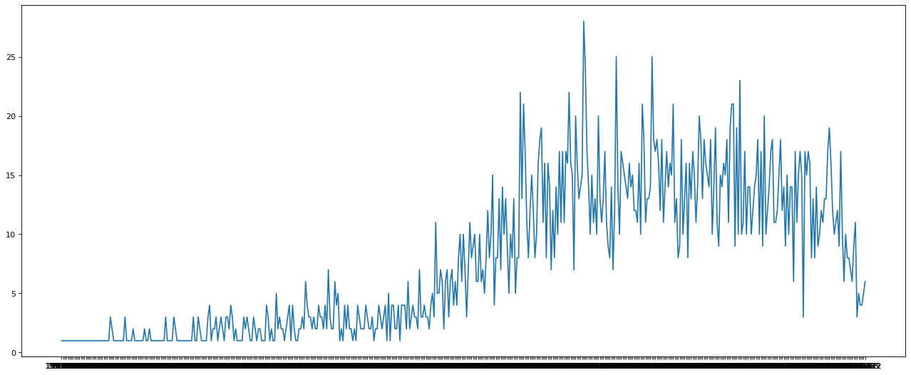
电影产量年份趋势

from matplotlib import pyplot as plt 
import random
from matplotlib import font_manager

movie_years = data.groupby('title_year')['movie_title']
print(movie_years.count().index.tolist()) 
print(movie_years.count().values)

---
['1927-02', ..., '2016-12']
[ 1  ... 6]

最后，我们利用之前学过的matplotlib进行数据可视化展示：

x = movie_years.count().index.tolist()
y = movie_years.count().values
plt.figure(figsize=(20,8),dpi=80)
plt.plot(x,y)
plt.show()

20231226135446

结尾

那小伙伴们，到今天为止，我们《AI 秘籍》系列课程中的「Python 部分」也就完全讲完了。就如我一开始向大家承诺的，这部分内容将完全免费。

而我们的《AI 秘籍》课程也才刚刚开始，未来很长一段时间内，我们都将继续和这些基础内容频繁打交道。用它们来呈现我们之后要用到的所有课程。包括 AI 基础，CV，BI，NLP 等课程。

不过在结束了一个阶段之后，我需要花点时间休整一下，也是为了好好的备课，找到最好的结构和顺序为大家编写后面的课程。本次课程的最后这两节课我都有些疲劳，为了赶快完成进度，编写过程当中可能有些粗糙或者遗漏，也请大家多包涵。日后，我可能会对这两节课进行更新，将一些细节的讲解补充完整。

免费部分结束了，日后的收费课程，也期望大家能一如即往的支持。

在这里，我也给大家推荐一些比较好的书籍，希望看到小伙伴们能够快速成长起来。

感谢大家，好了。本节课到此结束，下课了。

至此，Python 篇也结束了，欢迎大家关注「茶桁的 AI 秘籍」后续课程。