CNN

The source code: example_09: CNN

CNN Principle

1
2
3
4
5
6
7
8
9
10
11
12
import numpy as np
import pandas as pd
import matplotlib.pyplot as plt
from struct import unpack
from torchvision.datasets import MNIST
from sklearn.linear_model import LogisticRegression
import torch
from PIL import Image
from torch import nn

mnist_dataset_train = MNIST(root = '~/data/course_data', train=True, download = True)
mnist_dataset_test = MNIST(root = '~/data/course_data', train=False, download = True)

The first machine vision problem: Let the computer automatically distinguish between 0 and 6

1
2
3
4
5
6
7
8
9
10
11
12
X_train = mnist_dataset_train.data.numpy()
y_train = mnist_dataset_train.targets.numpy()

X_test = mnist_dataset_test.data.numpy()
y_test = mnist_dataset_test.targets.numpy()
"""
Downloading http://yann.lecun.com/exdb/mnist/train-images-idx3-ubyte.gz
Downloading http://yann.lecun.com/exdb/mnist/train-images-idx3-ubyte.gz to ~/data/course_data/MNIST/raw/train-images-idx3-ubyte.gz
9913344it [00:02, 4759648.85it/s]
...
5120it [00:00, 12492633.21it/s]Extracting ~/data/course_data/MNIST/raw/t10k-labels-idx1-ubyte.gz to ~/data/course_data/MNIST/raw
"""

Explain CNN principles

1
2
3
4
5
6
7
8
9
10
11
12
13
14
15
16
17
18
19
20
21
22
23
24
25
26
27
28
29
30
31
32
33
34
35
36
37
38
39
40
41
42
43
44
45
46
47
48
49
50
51
52
53
54
55
56
57
58
59
60
61
62
63
64
65
66
67
68
69
70
71
72
73
74
75
76
77
78
79
80
81
82
83
84
85
86
87
88
89
90
91
92
93
94
95
96
97
98
99
100
101
102
103
104
105
106
107
108
109
110
111
112
113
114
115
116
117
118
119
120
121
122
123
124
125
126
127
128
129
130
131
132
133
134
135
136
137
138
139
140
def conv(image, filter_):
# Convolution operation
print(image.shape)
print(filter_.shape)
assert image.shape[-1] == filter_.shape[-1]

test_image = image
height, width = filter_.shape[0], filter_.shape[1]

filter_result = np.zeros((
test_image.shape[0]-height + 1,
test_image.shape[1]-width + 1
))

for h in range(test_image.shape[0]-height + 1):
for w in range(test_image.shape[1]-width + 1):
sub_windows = test_image[h: h + height, w: w + width, :]
op = np.sum(np.multiply(sub_windows, filter_))

filter_result[h][w] = op

return filter_result

# Part 2: Strides
"""
Try to modify stride in Conv Function
"""
# Part3: Pooling
"""
Create a pooling cell for conv
"""
# Part4: Volume
"""
Create 3-d volume filter
"""
# Part5: Fully Connected Layers
"""
Create Fully Connected Layer, to flatten
"""
# Part6: Cross-Entropy
"""
Create Cross-Entropy cell to get loss value
"""
# Part7: ResNet
"""
Why we need resNet, and its functions
"""

class ResBlock(nn.Module):
"""
A very basic ResNet unit
The unit passed:
batch normal
The output value retains the original input value, so that our result does not dissipate
"""
def __init__(self, n_channel):
super(ResBlock, self).__init__()
self.conv = nn.Conv2d(n_channel, n_channel, kernel_size = 3, padding=1, bias = False)
self.bath_norm = nn.BatchNorm2d(num_features = n_channel)

torch.nn.init.constant_(self.bath_norw.weight, 0.5)
torch.nn.init.zeros_(self.bath_norm.bias)
torch.nn.init.kaiming_normal_(self.conv.weight, nonlinearity ='relu')
# sum(windows * filter) ==> The larger the windows, the larger the added value, the smaller the windows, the smaller the value

def forward(self, x):
out = self.conv(x)
out = self.conv(out)
out = self.bath_norm(out)
out = torch.relu(out)

return out + x

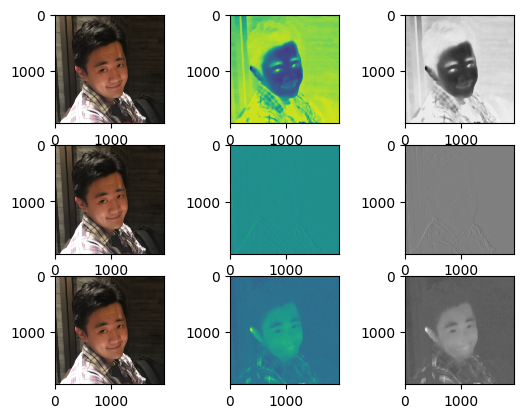
if __name__ == '__main__':
image = Image.open('~/data/course_data/doo.jpeg')

image_array = np.array(image)
plt.imshow(image_array)

# Robert 算子
rebert_1_kernel = np.array([
[1, 0],
[0, -1]
])
robert_2_kernel = np.array([
[0, 1],
[-1, 0]
])

#Sobel 算子
sobel_x_kernel = np.array([
[-1, 0, 1],
[-2, 0, 2],
[-1, 0, 1]
])
sobel_y_kernel = np.array([
[-1, -2, -1],
[0, 0, 0],
[1, 2, 1]
])

# Laplacian 算子
laplacian_kernel = np.array([
[0, 1, 0],
[1, -4, 1],
[0, 1, 0]
])

filters = [
np.array([sobel_x_kernel] * 3),
np.array([sobel_y_kernel] * 3),
np.array([laplacian_kernel] * 3)
]

for i, f in enumerate(filters):
print('applying filter: {}'.format(i))

plt.subplot(3, 3, i * 3 + 1)
plt.imshow(image_array)

filter_result = conv(image_array, f)
plt.subplot(3, 3, i * 3 + 2)
plt.imshow(filter_result)

plt.subplot(3, 3, i * 3 + 3)
plt.imshow(filter_result, cmap = 'gray')

plt.show()
#ResNet
"""
applying filter: 0
(1931, 1931, 3)
(3, 3, 3)
applying filter: 1
(1931, 1931, 3)
(3, 3, 3)
applying filter: 2
(1931, 1931, 3)
(3, 3, 3)
"""

output

Identification codes

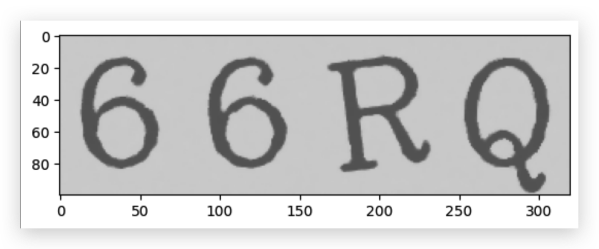
Train a model to classify and recognize the characters in the verification code, and finally complete the verification code recognition

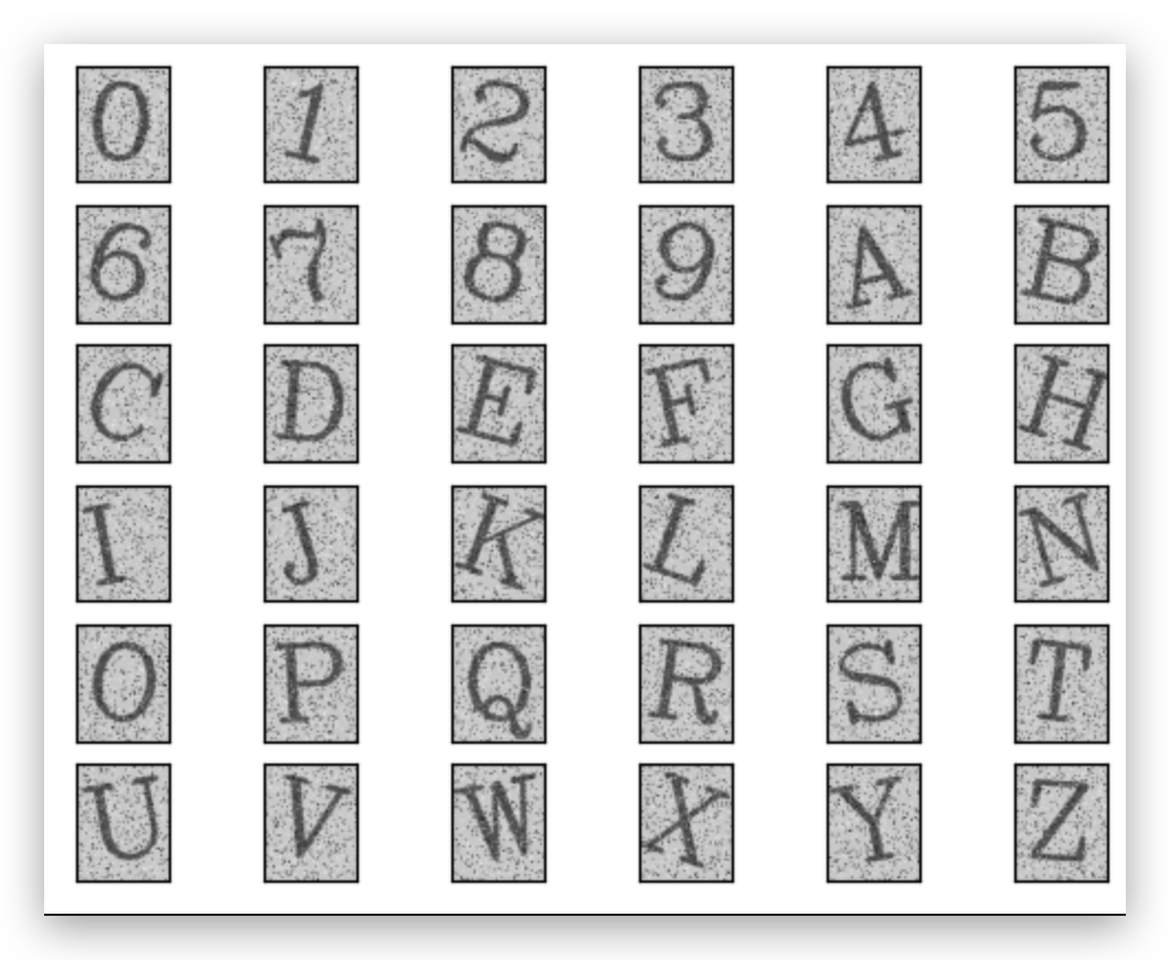
The data set used contains a total of 36 characters from 0-9 and AZ. There are 50 pictures for each character in the training set, and 10 pictures for each character in the verification set. The verification 
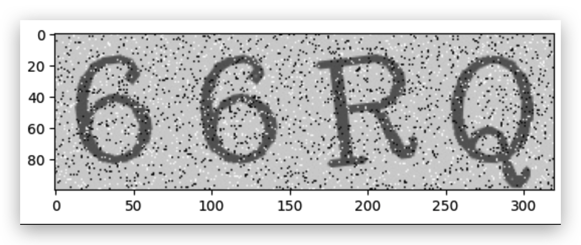
code data set is composed of 4 character pictures taken out randomly. become.

  1. Data Reading
  2. Use torch to build, train, and verify models
  3. Model prediction and image segmentation

analyze

Question 1-Establish a character comparison table

We can reverse each pair of keys and values by traversing the dictionary and store them in a new dictionary. The sample code is as follows:

1
new_dict = {v: k for k, v in old_dict.items()}
#### Question 2-Define datasets and dataloader In opencv-python, you can use image = cv2.medianBlur(image, kernel_size) for median filtering. #### Question 3-Define the network structure In torch, the convolution and fully connected layers are defined as follows:
1
2
conv = nn.Conv2d(in_channels, out_channels, kernel_size, stride, padding)
fc = nn.Linear(in_features, out_features, bias)
#### Question 4-Define the model training function The model training process of the torch framework includes operations such as clearing the gradient, forward propagation, calculating the loss, calculating the gradient, and updating the weight, among which: 1. Clear the gradient: the purpose is to eliminate the interference between step and step, that is, use only one batch of data loss to calculate the gradient and update the weight each time. Generally can be placed first or last; 1. Forward propagation: use a batch of data to run the process of forward propagation to generate model output results; 1. Calculate the loss: use the defined loss function, model output results and label to calculate the loss value of a single batch; 1. Calculate the gradient: According to the loss value, calculate the gradient value required in this optimization in the ownership of the model; 1. Update weight: Use the calculated gradient value to update the value of all weights. The sample code of a single process is as follows:
1
2
3
4
5
>>> optimizer.zero_grad() # Clear the gradient (can also be placed in the last line)
>>> output = model(data) # forward propagation
>>> loss = loss_fn(output, target) # Calculate loss
>>> loss.backward() # Calculate the gradient
>>> optimizer.step() # update weight

Programming

Import the library to be used in this project

1
2
3
4
5
6
7
8
9
10
11
12
13
14
15
import os
import cv2
import torch
import torch.nn as nn
import torch.nn.functional as F
import torch.optim as optim
from torch.utils.data import Dataset, DataLoader
import torchvision
import torchvision.transforms as transforms
import numpy as np
import pickle
import PIL
import matplotlib.pyplot as plt
from PIL import Image
os.environ['KMP_DUPLICATE_LIB_OK'] = 'True'

Understanding the data set

Define the data path

1
2
3
train_data_dir = '~/data/course_data/train_data.bin'
val_data_dir = '~/data/course_data/val_data.bin'
verification_code_dir = '~/data/course_data/verification_code_data.bin'

The data set used is stored in a binary file, and we need to define a function to read the picture in the binary file.

1
2
3
4
def load_file(file_name):
with open(file_name, mode ='rb') as f:
result = pickle.load(f)
return result

See what the data set looks like:

1
2
3
4
5
6
7
8
9
10
11
12
train_data = load_file(train_data_dir)
img_test = list()
for i in range(1, 1800, 50):
img_test.append(train_data[i][1])
plt.figure()

for i in range(1, 37):
plt.subplot(6, 6, i)
plt.imshow(img_test[i-1])
plt.xticks([])
plt.yticks([])
plt.show()

image-20210901131659902

View single big picture

1
2
3
4
5
# plt.subplot(6, 6, i)
plt.imshow(train_data[500][1])
plt.xticks([])
plt.yticks([])
plt.show()

image-20210901131741884

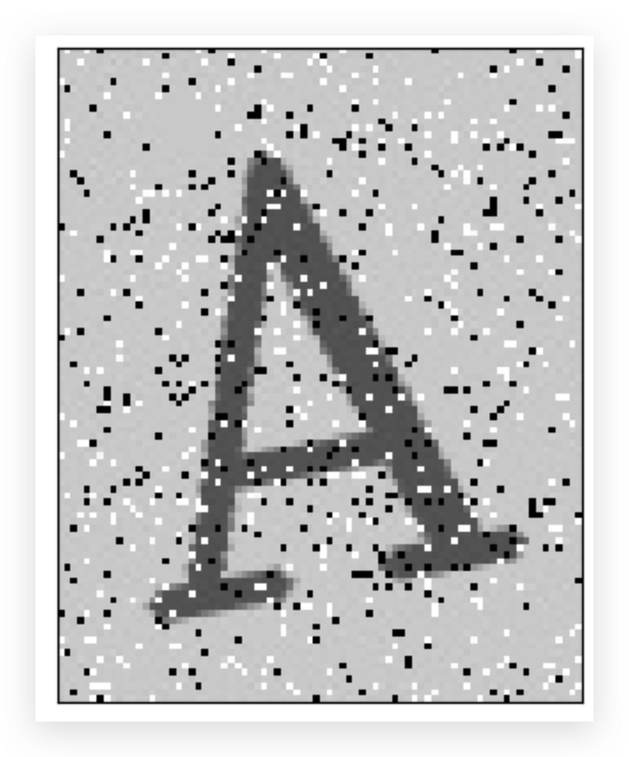
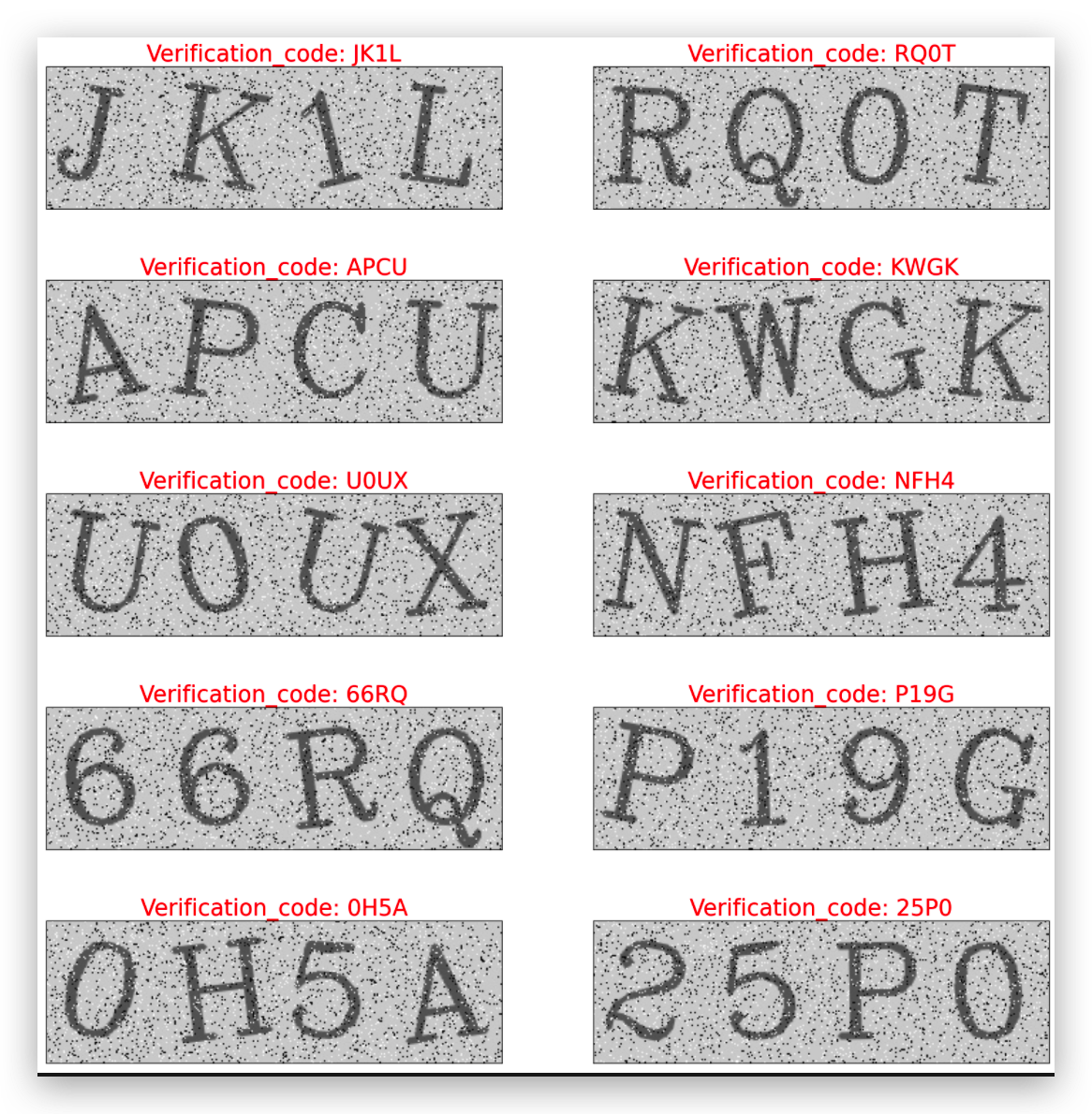
It can be seen that there is a lot of noise in the character picture, and the noise will have an adverse effect on the model prediction result, so we can use a specific filter to eliminate the picture noise during data preprocessing.

Question 1-Establish a character comparison table

A simple observation shows that there are no duplicates in the key and value in the character dictionary just defined. Therefore, the key and value in the dictionary can be reversed so that we can use the value to find the key (convert the model prediction result into a readable character) Now you need to complete the following code to reverse the keys and values in the dictionary (for example: dict={'A':10,'B':11} and get new_dict={10:'A ',11:'B'}

1
2
3
4
5
char_dict = {'0':0,'1':1,'2':2,'3':3,'4':4,'5':5,'6':6,'7':7,'8':8,'9':9,\
'A':10,'B':11,'C':12,'D':13,'E':14,'F':15,'G':16,'H':17,'I':18,'J':19,'K':20,'L':21,'M':22,\
'N':23,'O':24,'P':25,'Q':26,'R':27,'S':28,'T':29,'U':30,'V':31,'W':32,'X':33,'Y':34,'Z':35 }

new_char_dict = {v : k for k, v in char_dict.items()}

Question 2-Define datasets and dataloader

We need to use torch.utils.data.Dataset as the parent class to define our own datasets in order to standardize our own datasets.

1
2
3
4
5
6
7
8
9
10
11
12
13
14
15
class iDataset(Dataset):
def __init__(self, file_name, transforms):
self.file_name = file_name # file name
self.image_label_arr = load_file(self.file_name) # read binary file
self.transforms = transforms # Image converter

def __getitem__(self, index):
label, img = self.image_label_arr[index]
img = cv2.cvtColor(img, cv2.COLOR_RGB2GRAY) # Convert the picture to grayscale
img = cv2.medianBlur(img, 5) # Use median blur to remove image noise
img = self.transforms(img) # Transform the image
return img, char_dict[label[0]]

def __len__(self):
return len(self.image_label_arr)

Now we can define transform and dataloader.

1
2
3
4
5
6
7
8
9
10
transform = transforms.Compose([transforms.ToPILImage(),
transforms.Resize([28, 28]), # Adjust the image size to 28*28
transforms.ToTensor(), # Convert the picture to tensor
transforms.Normalize(mean = [0.5], std = [0.5])]) # Perform normalization processing

train_datasets = iDataset(train_data_dir, transform)
train_loader = DataLoader(dataset=train_datasets, batch_size=32, shuffle = True)

val_datasets = iDataset(val_data_dir, transform)
val_loader = DataLoader(dataset=val_datasets, batch_size = 32, shuffle = True)

Question 3-Define the network structure

After the data is ready, we need to define a simple convolutional neural network. The input of the neural network is [batchsize,chanel(1),w(28),h(28)], and the output is 36 categories. Our neural network will use 2 convolutional layers with 2 fully connected layers. The parameter settings of these four layers are shown in the following table (the default parameters can be used directly if they are not marked): 1. conv1: in_chanel=1, out_chanel=10, kernel_size=5 1. conv2: in_chanel=10, out_chanel=20, kernel_size=3 1. fc1: in_feature=2000, out_feature=500 4. fc2: in_feature=500, out_feature=36

1
2
3
4
5
6
7
8
9
10
11
12
13
14
15
16
17
18
19
20
21
22
23
class ConvNet(nn.Module):
def __init__(self):
super().__init__()
# TODO:
self.conv1 = nn.Conv2d(1, 10, 5)
self.conv2 = nn.Conv2d(10, 20, 3)
self.fc1 = nn.Linear(20 * 10 * 10, 500)
self.fc2 = nn.Linear(500, 36)

def forward(self, x):
# inputsize: [b, 1, 28, 28]
in_size = x.size(0) # b
out = self.conv1(x)
out = F.relu(out)
out = F.max_pool2d(out, 2, 2)
out = self.conv2(out)
out = F.relu(out)
out = out.view(in_size, -1)
out = self.fc1(out)
out = F.relu(out)
out = self.fc2(out)
out = F.log_softmax(out, dim = 1)
return out

Question 4-Define the model training function

Next, we need to complete the model training function to achieve the following operations: 1. Clear the gradient 1. Forward propagation 1. Calculate the gradient 1. Update weights

1
2
3
4
5
6
7
8
9
10
def train(model, train_loader, optimizer, epoch):
model.train()
for batch_idx, (data, target) in enumerate(train_loader):
optimizer.zero_grad()
output = model(data)
loss = F.nll_loss(output, target)
loss.backward()
optimizer.step()
if(batch_idx + 1) % 10 == 0:
print('Train Epoch: {} [{} / {} ({:.0f} %)]\tLoss: {:.6f}'.format(epoch, batch_idx * len(data), len(train_loader.dataset), 100. * batch_idx / len(train_loader), loss.item()))
Define model test function
1
2
3
4
5
6
7
8
9
10
11
12
def test(model, test_loader):
model.eval()
test_loss = 0
correct = 0
with torch.no_grad():
for data, target in test_loader:
output = model(data)
test_loss += F.nll_loss(output, target, reduction = 'sum')
pred = output.max(1, keepdim = True)[1]
correct += pred.eq(target.view_as(pred)).sum().item()
test_loss /= len(test_loader.dataset)
print('\nTest set: Average loss: {:.4f}, Accuracy: {}/{} ({:.0f}%) \n'.format(test_loss, correct, len(test_loader.dataset), 100. * correct / len(test_loader.dataset)))
Define model and optimizer

We define the model structure we just built as model and choose to use the Adam optimizer.

1
2
model = ConvNet()
optimizer = optim.Adam(model.parameters())
Model training and testing

We can first set the number of epochs to 3 and perform model training to see how accurate the model is and whether it meets the requirements of verification code recognition. If the model accuracy is not enough, you can also try to adjust the number of epochs and retrain.

1
2
3
4
5
6
7
8
9
10
11
12
13
14
15
16
17
18
19
20
21
22
23
24
25
26
27
28
29
30
EPOCHS = 3
for epoch in range(1, EPOCHS + 1):
train(model, train_loader, optimizer, epoch)
test(model, val_loader)

"""
Train Epoch: 1 [288 / 1800 (16 %)] Loss: 3.340514
Train Epoch: 1 [608 / 1800 (33 %)] Loss: 2.872326
Train Epoch: 1 [928 / 1800 (51 %)] Loss: 1.977929
Train Epoch: 1 [1248 / 1800 (68 %)] Loss: 1.098688
Train Epoch: 1 [1568 / 1800 (86 %)] Loss: 0.535660

Test set: Average loss: 0.2888, Accuracy: 328/360 (91%)

Train Epoch: 2 [288 / 1800 (16 %)] Loss: 0.072813
Train Epoch: 2 [608 / 1800 (33 %)] Loss: 0.139866
Train Epoch: 2 [928 / 1800 (51 %)] Loss: 0.109487
Train Epoch: 2 [1248 / 1800 (68 %)] Loss: 0.058259
Train Epoch: 2 [1568 / 1800 (86 %)] Loss: 0.013144

Test set: Average loss: 0.0099, Accuracy: 360/360 (100%)

Train Epoch: 3 [288 / 1800 (16 %)] Loss: 0.010245
Train Epoch: 3 [608 / 1800 (33 %)] Loss: 0.004797
Train Epoch: 3 [928 / 1800 (51 %)] Loss: 0.002203
Train Epoch: 3 [1248 / 1800 (68 %)] Loss: 0.006250
Train Epoch: 3 [1568 / 1800 (86 %)] Loss: 0.005230

Test set: Average loss: 0.0028, Accuracy: 360/360 (100%)
"""
Define model test function
1
2
3
4
5
6
7
8
9
10
11
12
def test(model, test_loader):
model.eval()
test_loss = 0
correct = 0
with torch.no_grad():
for data, target in test_loader:
output = model(data)
test_loss =+ F.nll_loss(output, target, reduction = 'sum')
pred = output.max(1, keepdim = True)[1]
correct += pred.eq(target.view_as(pred)).sum().item()
test_loss /= len(test_loader.dataset)
print('\nTest set: Average loss: {:.4f}, Accuracy : {}/{} ({:.0f}%) \n'.format(test_loss, correct, len(test_loader.dataset), 100. * correct / len(test_loader.dataset)))
Define model and optimizer

We define the model structure we just built as model and choose to use the Adam optimizer.

1
2
model = ConvNet()
optimizer = optim.Adam(model.parameters())
Model training and testing

We can first set the number of epochs to 3 and perform model training to see how accurate the model is and whether it meets the requirements of verification code recognition. If the model accuracy is not enough, you can also try to adjust the number of epochs and retrain.

1
2
3
4
5
6
7
8
9
10
11
12
13
14
15
16
17
18
19
20
21
22
23
24
25
26
27
28
29
EPOCHS = 3
for epoch in range(1, EPOCHS + 1):
train(model, train_loader, optimizer, epoch)
test(model, val_loader)
"""
Train Epoch: 1 [288 / 1800 (16 %)] Loss: 3.508450
Train Epoch: 1 [608 / 1800 (33 %)] Loss: 3.288610
Train Epoch: 1 [928 / 1800 (51 %)] Loss: 2.584805
Train Epoch: 1 [1248 / 1800 (68 %)] Loss: 1.180833
Train Epoch: 1 [1568 / 1800 (86 %)] Loss: 0.564084

Test set: Average loss: 0.0088, Accuracy : 316/360 (88%)

Train Epoch: 2 [288 / 1800 (16 %)] Loss: 0.173177
Train Epoch: 2 [608 / 1800 (33 %)] Loss: 0.043262
Train Epoch: 2 [928 / 1800 (51 %)] Loss: 0.054462
Train Epoch: 2 [1248 / 1800 (68 %)] Loss: 0.052596
Train Epoch: 2 [1568 / 1800 (86 %)] Loss: 0.013714

Test set: Average loss: 0.0006, Accuracy : 360/360 (100%)

Train Epoch: 3 [288 / 1800 (16 %)] Loss: 0.004590
Train Epoch: 3 [608 / 1800 (33 %)] Loss: 0.007654
Train Epoch: 3 [928 / 1800 (51 %)] Loss: 0.004135
Train Epoch: 3 [1248 / 1800 (68 %)] Loss: 0.003140
Train Epoch: 3 [1568 / 1800 (86 %)] Loss: 0.003019

Test set: Average loss: 0.0001, Accuracy : 360/360 (100%)
"""

The model has been trained! Does the test set accuracy of the last epoch exceed 99%?

Identification codes

After successfully implementing the digital recognition, we can start the verification code recognition! First, import the verification code data set:

1
verification_code_data = load_file(verification_code_dir)

Let's choose a picture at random (Figure 6) to see what the verification code looks like.

1
2
3
4
image = verification_code_data[6]
IMG = Image.fromarray(cv2.cvtColor(image.copy(), cv2.COLOR_BGR2RGB))
plt.imshow(IMG)
plt.show()

image-20210901132522728

Let's take a look at what effect the median filter can have on the captcha image.

1
2
3
img = cv2.medianBlur(image.copy(), 5)
plt.imshow(img)
plt.show()

image-20210901132551457

Finally, let us look at the actual results of verification code recognition:

1
2
3
4
5
6
7
8
9
10
11
12
13
14
15
16
17
18
19
20
21
22
23
24
25
26
27
28
29
IMAGES = list()
NUMS = list()

for img in verification_code_data:
IMAGES.append(img)
img = cv2.cvtColor(img, cv2.COLOR_RGB2GRAY)
image_1 = img[:, :80]
image_2 = img[:, 80:160]
image_3 = img[:, 160:240]
image_4 = img[:, 240:320]
img_list = [image_1, image_2, image_3, image_4]

nums = []
for one_img in img_list:
one_img = transform(one_img)
one_img = one_img.unsqueeze(0)
output = model(one_img)
nums.append(new_char_dict[torch.argmax(output).item()])
NUMS.append('Verification_code: '+ ''.join(nums))

plt.figure(figsize = (20, 20))
plt.subplots_adjust(wspace = 0.2, hspace=0.5)
for i in range(1, 11):
plt.subplot(5, 2, i)
plt.title(NUMS[i-1], fontsize = 25, color = 'red')
plt.imshow(IMAGES[i - 1])
plt.xticks([])
plt.yticks([])
plt.show()

image-20210901132631369

作者

Hivan Du

发布于

2021-09-02

更新于

2023-06-02

许可协议

评论